
Robert Turley and Dr. James B McDonald, Economics
Traditional methods for estimating economic relationships assume the error between their predictions and their observations to be normally distributed. In other words, the random variable representing the error term is expected to follow the Gaussian distribution popularly known as the bell curve. In the case of a linear model, this is one of the justifications for the regression technique known as ordinary least squares (OLS). However, in many cases it appears the distribution of the error in economic models is peaked or skewed, suggesting that it may be inappropriate to assume normality.
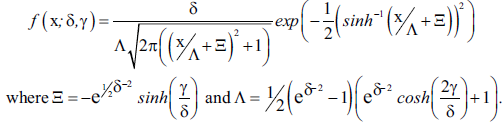
One method to account for non-normality is to use a probability density that has a very flexible shape, estimating its shape parameters concurrently with the parameters corresponding to the economic model using a technique known as quasi-maximum likelihood estimation (QMLE). The one-parameter Student’s t and the two-parameter EGB2 distributions have been used frequently in QMLE regression in recent econometric literature. This research examines an alternative two-parameter distribution based on the SU distribution suggested by Johnson.i This distribution is derived from the hyperbolic transformation of a normal random variable z, so that we consider x where z = ã + äsinh-1(x). This transformation suggests we refer to this distribution as the inverse hyperbolic sine (IHS). After appropriate location and scale changes for a zero mean and unitary variance, the probability density corresponding to our new random variable is
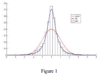
A chief advantage of using this distribution is its ability to model a variety of combinations of skewness and peakedness; the flexibility provided by its two shape parameters can be seen in figure 1 where the IHS and the normal distributions are fit to a probability histogram of the daily change in the dollar price of gold.
In examining the usefulness of QMLE methods using the IHS distribution, it is interesting to examine how much outliers caused by such factors as measurement error can bias estimation.
An estimators influence function is one method of quantifying this bias. Roughly speaking, a graph of the influence function shows how the magnitude of bias changes with respect to the magnitude of the outlier. OLS techniques have been shown particularly sensitive to outliers with a constantly increasing influence function, meaning a large outlier could greatly bias estimation. On the other hand, the influence function of the IHS estimator decreases. This suggests that IHS estimation will be more robust than least absolute deviations regression, which has a constant influence function. The influence function of the IHS closely resembles that of the Student’s t, an estimator considered to be very robust.
To test applications of IHS regression computer routines were written using the Matlab platform and incorporated into econometric programs used by James McDonald of the Department of Economics. It appears that these estimation techniques are both fast and efficient.
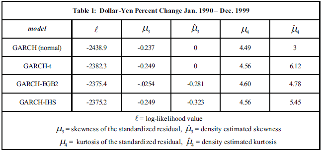
To compare the performance of the IHS against the normal, Student’s t and EGB2 distributions, each were used as the conditional density for the error in a Generalized Autoregressive Conditional Heteroskedasticity (GARCH) model of financial volatility.ii Judging by the goodness-of-fit measures seen in table 1, the IHS clearly outperforms the normal and Student’s t densities, with a greater likelihood value and skewness and kurtosis estimates that are much closer to the sample. Although the IHS has a slightly greater log-likelihood value than the EGB2, it does slightly worse in modeling the skewness and kurtosis. It is unclear which of the two would be considered a better model of the data.
This research suggests that the IHS distribution has great potential for modeling non-normal data, performing at least as well as other flexible distributions currently being considered in econometric research.
________________________________________
i Johnson, N.L., 1949, “Systems of Frequency Curves Generated by Methods of Translation,” Biometrika 36.
ii The GARCH-EGB2 model was introduced in Wang, Kai-Li, Christopher Fawson, Christopher Barrett, and James McDonald, 2001, “A Flexible Parametric Garch Model with an Application to Exchange Rates,” Journal of Applied Econometrics 16: 521-536.