
Blair R. Brown and Dr. Earl M. Woolley, Chemistry and Biochemistry
In Dr. Woolley’s lab we have made extensive measurements of the Apparent Molar Heat Capacities of aqueous solutions using a Nano Differential Scanning Calorimeter, N-DSC (Calorimetry Science Corporation, Spanish Fork, UT). Through modifications to the N-DSC we are now able to do pressure perturbation calorimetry. That is to say we may now change the pressure of a solution and measure the change in the heat of that solution, (dq/dP)T ( as opposed to (dq/dT)p which is heat capacity). This property is related to entropy by the 2nd law of thermodynamics in the following way (dq/dP)T = T(dS/dP)T. From a Maxwell relation we see that (dS/dP)T = -(dV/dT)p which is defined as expansibility. In combining the two relationships we obtain (dq/dP)T = -T(dV/dT)p, therefore by measuring how the heat changes as we change the pressure of a solution we may obtain expansibility.
Our first task was to determine whether or not we could obtain reproducible heat signals using our N-DSC. Solutions of NaCl(aq) and KHP(aq) were prepared by weight using distilled, deionized, degassed, and autoclaved water. Calorimetric runs are conducted by filling the sample cell with the solution of interest and the reference cell with pure water. The heat signal obtained in this manner is a differential signal, which is the difference between the response of the sample, and the response of water, to the pressure change. As a result it is necessary to subtract the effects of the non-uniformity of the two cells. To accomplish this we ran water in both cells to obtain a signal and then subtracted this signal from the signal obtained with an actual sample. Multiple runs were conducted of NaCl(aq), KHP(aq), and water under varying experimental parameters in order to find the optimal way to conduct pressure scans. Through this experimentation we discovered the optimal run consisted of the following. The pressure was varied between 2 and 5 atm, with 4 up scans (2-5) and 4 downs scans (5-2). Each pressure change was effected over a 3 minute 20 second period with a subsequent 10 minute recovery period in order for the calorimeter to measure the total heat response from the pressure change. After the ten minute period the pressure would again be changed, this time in the opposite fashion. The run was started off with a non-used up scan to equilibrate the instrument and then the eight usable scans were performed. This was all performed at one temperature, once completed the temperature was increased and another run was performed. Samples were run from 5 to 115 degrees C in 10 degree increments. For each temperature the run took 3 hours and 20 minutes to complete and with 10 temperatures per sample it took approximately a day and a half to run on sample. Multiple concentrations were also run for each solution studied. With these optimized run conditions we then obtained usable data for the different solutions.
The next problem we encountered was obtaining, from the raw data, the total heat change resultant from the pressure change. In order to accomplish this I programmed a macro in Microsoft excel that would calculate the area under the plot of heat signal vs. time; this value is the total heat change, dq, for each pressure change, dP.
Next came the hardest part of the whole process, calibrating the calorimeter to give the correct value for expansibility. There are a few problems associated with calibration. First it requires that we use two solutions with know expansibilities to obtain a calibration constant for our equation. Apparent molar expansibilities, the expansibility of the sample compared to that of water, will become zero at the temperature where the sample’s expansibility equals that of water. When this value goes to zero there will be no heat signal and we can not obtain a calibration constant for that temperature. Therefore by using two different calibration solutions we may obtain the calibration constant for all temperatures. This is why both KHP and NaCl were used to perform the calibration experiments. The next problem is that in order to know the expansibilities of our standards we must take the derivatives of their apparent molar volume surfaces. The difficulty of taking this derivative introduces a large source of error. Also there is the argument that if we are taking derivatives of the volumes of our standard solutions to obtain their expansibilities then why not do this for all solutions and not bother with the pressure perturbation calorimetry in the first place.
Calibration runs were carried out with 0.99944 mol∙kg-1 NaCl(aq) and 0.486919 mol∙kg-1 KHP(aq). Water runs were carried out after every two sample runs. The equation we used in order to obtain calibration constants, k, as well as calculate expansibilities of samples is as follows.
![]()
In this equation the subscript s and the subscript w refer to sample and water, respectively. By using this equation we obtained calibration constants for both NaCl(aq) and KHP(aq). Then using these calibration constants we tried to reproduce the expansibilities for the other standard to see if we are getting the right answer. Simply put we used the calibration constants for NaCl(aq) to reproduce the expansibilities for KHP(aq) and vice versa. The table below contains our results.
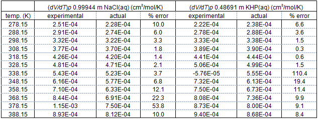
The temperatures with high errors correlate to those regions where the calibrant’s apparent molar expansibility is equal to zero. The other errors are due to problems with taking derivatives, with area calculations, reproducibility of runs, and accuracy of water runs. Our future efforts will be directed at improving these problems and reducing this error to acceptable levels.