Randall Lewis and Dr. James McDonald, Economics

In the field of economics, the estimation of causal relationships is fundamental. The economist formulates a model or mechanism through which human behavior affects outcomes. Then, by using real-world data, economists can estimate these relationships. For example, one simple relationship that has been a subject of study is the causal effect of education on income. Whereas in other fields correlation is typically the object of interest, in economics, the actual quantitative effect on outcomes of changing a causal variable, such as years of education, is of interest.

In order to determine the average effect of changing a variable by one unit, data gathered from a representative sample can be used to estimate a relationship such as log(Income) = β1 + β2*YearsEducation. One technique which has become the workhorse of economic analysis is ordinary least squares (OLS) estimation. OLS estimates a linear relationship by obtaining the “best fit” of the data through minimizing the square of the residuals, the differences between the actual observations and the model’s predictions.

Several assumptions are made implicitly when using least squares and performing statistical inference on the estimated model. Three assumptions are homoskedasticity, no serial correlation, and normality of the residuals. Econometricians have formulated methods to account for these issues. Another possible problem in the data is censoring, where a threshold is observed instead of the actual value of the variable (observations such as “income is greater than $80,000”). Data censoring of the outcome variable exacerbates the three problems mentioned above. In fact, while OLS is the best way to obtain the model estimates (a minimum variance unbiased estimator), under censoring, it can be far from the true relationship, a condition known as bias. Amemiya (1978) has shown that when the sample size grows quite large, the tobit model proposed by Tobin (1958) gives consistent results and thus solves the problem of data censoring, as long as none of the three assumptions above are violated.

Unfortunately, when any one of the three assumptions above are violated, it has been shown that the tobit model is not necessarily reliable. Researchers have attempted to address each of these problems. In our research, we addressed the problem of nonnormality of the residuals in order to provide a better estimation method.

The method that we implemented and tested against various alternatives is known as quasi-maximum likelihood estimation (QMLE). QMLE uses the advantages of maximum likelihood estimation while allowing for residual distribution flexibility. By using several families of probability density functions that have the normal distribution as a special case, QMLE also allows for nested hypothesis testing and includes the tobit as a special case. This helps guard against overfitting (making the model fit the data), which reduces the model’s predictive power.

The distribution families that we used were the skewed generalized t (SGT), exponential generalized beta of the second kind (EGB2), and inverse hyperbolic sine (IHS). To test the QMLE using these distribution families, we estimated a model of out of pocket health care expenditures and performed a simulation study where we randomly generated thousands of datasets to test the performance of the estimators. We also included the censored least absolute deviation (CLAD), Heckman, and semiparametric least squares (SP-LS) estimators in our comparison against the OLS, non-censored least squares (NC-OLS), and tobit estimators.

The results from the out of pocket health care expenditures model suggest that the residuals are not normally distributed (above left) and that the tobit model produces substantially different results from those of the models that allow for skewness and thick tails in the residual distribution (above right). CLAD, which has been shown to perform quite well under general conditions, also has substantially different results from the tobit. Thus, given the nonnormality of the residuals, one would be better off using one of the alternative methods.

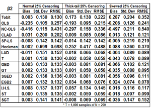
The simulation study corroborated the health care example results by showing that under normality, the tobit model does the best. But, upon introducing nonnormality in the residuals, the other models performed far better by reducing the bias and variability of the estimate. Thick-tailed and skewed residuals both greatly diminished the usefulness of the tobit in producing reliable results. The other models did much better, with the QMLE models performing the best in terms of mean squared error.

In conclusion, if one is willing to use the tobit to estimate a model, it may prove useful to also estimate the model using these QMLE methods to determine whether the assumption of normality is reasonable. As in the health care expenditure model, one of the other methods may provide more reliable results with more valid inference.

References

• Amemiya, T., 1973. “Regression Analysis when the Dependent Variable is a Truncated Normal.” Econometrica, 41, 997-1016.
• Tobin, J., 1958. “Estimation of Relationships for Limited Dependent Variables.” Econometrica, 26, 24-36.