Casey Abbott and Dr. John Hedengren, Department of Chemical Engineering

Advances in biomedical research have lead to an increase of experimental data to be interpreted in the context of reaction pathways, molecular transport, and population dynamics. Kinetic modeling is one way employed to interpret this data and is used in the pharmaceutical industry in developing clinical trials for new medications [1]. One collection of kinetic models is built on the System Biology Markup Language (SBML). Many of these models have detailed reaction metabolic pathways that describe biological systems, including cause and effect relationships in the human body. While simulations of these biological systems have been successfully applied for many years, the alignment to available measurements continues to be a challenge. The best available solution techniques continue to limit the size of models and measurements to small and medium size problems.

Recent developments may have changed this situation: an optimization technique known as the simultaneous approach has shown promise in efficiently optimizing large models (thousands of variables and parameters) [2]. In this method, the model and optimization problem are solved simultaneously, as opposed to the traditional approach of solving the differential and algebraic equations (DAE) model sequentially. Much of the recent development for the simultaneous approach has occurred in the petrochemical industry, where on-line process control applications require optimization of nonlinear models with many decision variables in the span of minutes. Using the same solution techniques, major advances in the biological systems area are possible. One software that takes advantage of the simultaneous approach is APMonitor (APM).

To verify that APM can accurately simulate biological models it was used to simulate a toy model and the results were compared to literature values. The model used is a basic model describing the HIV virus over thirty days with nine parameters, three variables and three differential equations [3]. APM was successfully able to replicate the results published in the literature. Once it was shown that APM could simulate biological models accurately the next step was to verify the parameter estimation capabilities of APM. This was done using a HIV model similar to those mentioned above. In order to perform the parameter estimation the objective function was set to minimize the absolute error between the model and synthetic data. There was measurement noise of plus or minus 0.5 log order added to the synthetic data. It was found that APM was able to accurately find the correct values for all six parameters.

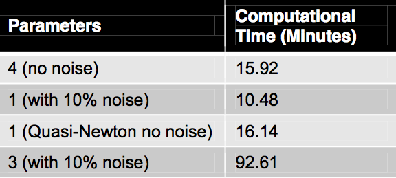
Once APM’s capabilities were verified on the HIV models, they were applied to a model that describes the ErbB signaling pathways [4]. This model shall be referred to as the ErbB model. It is a large model with 225 parameters, 504 variables and 1331 DAEs. In the article the authors estimated 75 of the initial conditions and rate constants out of the 229 identified by the sensitivity analysis. This was accomplished through simulated annealing which required 100 annealing runs and 24 hours on a 100-node cluster computer on average to obtain just one good fit. The APM simulation was not able to accurately replicate the literature values, but do show the dynamics found in the literature. It is believed that the discrepancy is due to an error in the conversion of the piecewise functions from the SBML model to the APM model. Even with the literature values not replicated exactly, parameter estimation was still preformed with the results shown in Table 1. The table gives the time for APM to solve the parameter estimation for the given number of parameters and amount of noise for the synthetic data. It also gives a value to a sequential Quasi-Newton solver with a BFGS update that was created to compare the sequential and simultaneous methods. The sequential method was able to estimate up to one parameter, while the simultaneous method was able to estimate up to four parameters with no noise. The last row in Table 1 gives the most realistic information. In this run, three parameters were estimated with 30 synthetic data points and noise comparable to that of the real data. The data given in Table 1 was generated on a personal PC with a single CPU. These results were presented at the annual AIChE Conference Nov. 1, 2012. [5]

Table 1

References

1. Adiwijaya, B. S. Herrmann, E. Hare, B. Kieffer, T. Lin, C. Kwong, A. D. Garg, Randle, J. C. R. Sarrazin, C. Zeuzem, S. and Caron, P. R. (2010), “A Multi-Variant, viral dynamic model of genotype 1 HCV to assess the in vivo evolution of protease-inhibitor resistant variants,” PLoS Comput. Biol., 6(4):e1000745.
2. Biegler, L. T. (2007), “An overview of simultaneous strategies for dynamic optimization,” Chemical Engineering and Processing: Process Intensification, 46(11) pp. 1043 – 1053.
3. Nowak, M. and May, R. (2000), Virus Dynamics Mathematical Principles of Immunology and Virology. Oxford, New York: Oxford University Press.
4. Chen, William W. Schoeberl, Birgit Jasper, Paul J. Niepel, Ulrik B. Lauffenburger, Douglas A. and Sorger, Peter K. (2009), “Input-output behavior of ErbB signaling pathways as revealed by a mass action model trainded against dynamic data,” Molecular Systems Biology, 5, pp. 239.
5. Acknowledgements: Dr. Eric Haseltine, David Grigsby and Abraham Martin