
Geraldine Hansen and Dr. C. Shane Reese, Statistics
Researchers and developers in manufacturing and industry are often confronted with the problem of testing component functionality. Two important testing methods used on equipment are destructive testing (DT) or nondestructive evaluation (NDE). DT implies that the part is destroyed by disassembly, or it is destroyed by utilizing the equipment to determine if the part was defective. In the case we examined, DT is like exploding a weapon. DT is very expensive and reduces valuable assets, but it is consistently very accurate. This type of testing is often referred to as obtaining a “snapshot in time” because we know at that instant (and at no other point in time) whether or not the equipment is working.
The other type of testing, NDE, is most often associated with techniques such as radiography, where an internal picture of the equipment is taken and then evaluated to predict if the equipment will work. This generally has lower cost and usually no reduction of assets, but the accuracy is often sacrificed, and unfortunately, often unknown. NDE is more informative than DT over a period of time because the functionality of parts can be evaluated again and again as the equipment ages. The benefits of NDE indicate the importance of considering it as a testing technique; however, the uncertainty with regard to NDE needs to be examined.
The proposal that we submitted indicated that we would examine a complex situation where a success weapon is evaluated on a continuous scale. However, in the past year, our research focus has been to perfect and more completely understand the case where an explosive is evaluated to be either a failure (mathematically denoted as 0) or success (denoted as 1). During the last few months, we have begun the more complex case, although at this time it is still in the developmental stages. The research we did allowed us to develop a statistical framework for comparison that can be generalized according to parameters that are given by researchers. This information was shared at the College of Physical and Mathematical Science’s Spring Research Conference, where it was recognized with a reward of merit.
This summer we produced a report that analyzes how nuclear weapon testing has changed and been affected by legislation in the United States, focusing on current rumors that nuclear testing may resume. This library-based research allowed us to connect our research with current issues. An outline of our procedure for creating the statistical framework follows, in which we make the comparison based on a simulation to estimate the probability that NDE detects a good part correctly. We employ the distributions of the two types of testing, and misclassification probabilities to create that simulation.
We assume DT data (X1,X2,Xn…, ) accurately reflects the probability of a good part. Furthermore, each test has an independent Bernoulli distribution (a useful distribution for modeling success/failure outcomes) with parameter p where = Pr( = 1) i p X , or the probability that a part functions as designed.
NDE data (Z1,Z2,Zn…, ) also has a Bernoulli distribution, but instead of success parameter p, NDE has success parameter p* where * = Pr( = 1) i p Z , or the probability of the test indicating a functional part. There are two misclassifications, or errors, that are associated with NDE and each of these is assigned a probability of occurring. Misclassification probabilities can be defined as the errors when NDE indicates a component is good when it actually is bad g b P | =Pr(Zi=1|Xi=0), or that a component is bad when it is, in fact, good b g P| =Pr(Zi=0|Xi=1). The NDE parameter p* can be shown to be equal to p* = b g g b p P p P | | (1- ) + (1- ) . Because p* incorporates the misclassification probabilities as well as what we know from the true probability, a comparison between the methods can then be achieved.
The parameter p (proportion of successes based on the DT data) can be shown to have a distribution which follows a Beta distribution (by simple application of Bayes Theorem). All distribution characteristics, such as means, standard deviations, and quantiles, can then be obtained analytically. However, the distribution of p* which is based on NDE data must be simulated through Markov Chain Monte Carlo (MCMC) methods since the form is unknown.
This process results in a generated distribution of p*. After generating thousands of distributions of the parameters p and p*, we compare the two different distributions by using the 90 percentile of each, so that the center and spread of the distributions are both accounted for. The practical application of this work is that the probability of success based on DT and the probability of success based on NDE can be compared. Using this comparison the number of NDE tests that must be done to reach the same uncertainty level (similar to “confidence level” in classical statistics) that DT gives you. Figure 1 shows the different number of tests for each method that are equivalent. The approximation of these points allows us to estimate that for however many DT tests that are required, we will need twice as many NDE tests to obtain the same level of confidence. This simulation was created as if the known probability was p =0.4167, and the misclassification probabilities were g b P | =0.35 and b g P| =.005, where all of these values were based on information from an actual NDE measurement process.
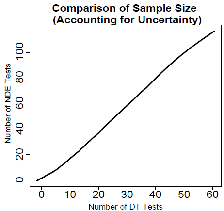
By slight modifications of code, we can examine the relationship between DT and NDE for a variety of choices of g b P | , b g P| , and p. Each situation would result in a new “equivalence” curve (like the one shown in Figure 1). These curves can be used by decision makers to decide if a shift to NDE is a worthwhile option.