
Zach White
An Algorithm for Multiple Regression Variable Selection for Biochemical Oxygen Demand
Dr. William Christensen Department of Statistics
Introduction
Biochemical Oxygen Demand (BOD) is used to measure of the amount of oxygen required by aerobic bacteria and other microorganisms to stabilize decomposable organic matter. It is run as a laboratory based biodegradation test and relies upon the presence of a thriving microbial community that may be naturally present in the sample or artificially introduced by addition of a seed, commonly a known volume of sewage effluent of known BOD. A standard BOD test is run in the dark at a temperature of 20 degrees Celsius for 5 days. This is defined as a five-day BOD (BOD5), which is the oxygen used in the first five days. Although BOD is the current standard, this test is not only long (five days),
but it also be cost-prohibitive in developing countries due to the cost of the equipment required.
Excitation Emission Matrix (EEM) is a test that measures
the fluorescence of a water sample and is created
by simultaneously scanning excitation and emission
wavelengths through an aqueous sample. EEM takes
less than two hours to produce results. So, this procedure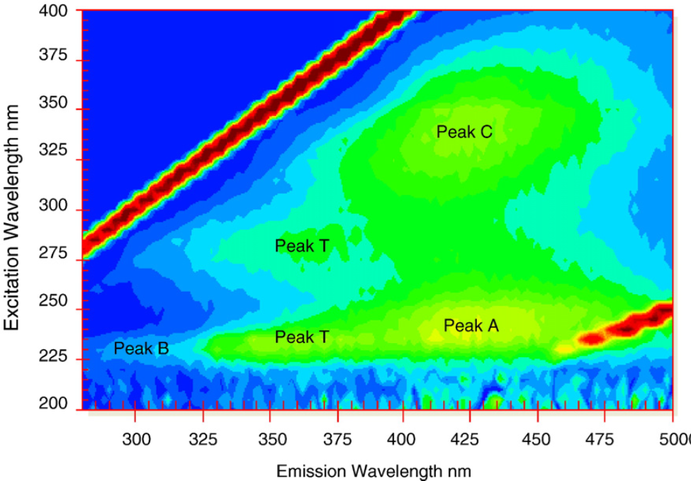 could be used to monitor water treatment processes
in real time, which isn’t possible with BOD5 because
of the length of the procedure. However, EEM is difficult
to interpret since it produces a 30×40 matrix with
1200 values. A visualization of an EEM is shown. Our
data consists of EEM matrices and corresponding BOD
measurements from four sites in the Provo waste water
treatment plant and 3 sites from the Orem waste water
treatment plant.
We seek to use multiple regression from multiple locations in the EEM matrix to predict BOD values. However, since the the data (155 observations) are so sparse relative to the number of variables (1200), the major obstacle to building a viable model is with so many more variables than observations, it is easy to overfit the model, which would result in not actually capturing the trend but rather juts
capturing the data we have. We seek to understand which locations of the EEM matrix are most predictive of BOD, which would make EEM more intrepretable. It would be a way to leverage the benefits of EEM with the stability and interpretability of BOD.
Research Strategy
1. In this algorithm, we start by fitting multiple regression models with 10 randomly chosen variables (this number was arbitrarility selected by the consulting civil engineering professor and graduate student). We fit 100,000 different models in this way. After these models are fit, we sort through these models and their respective R2 values. We keep the models whose R2 value is greater than an established percentile of all of the models’ R2 value. The variables of each model whose R2 value meets this criteria recieves a ”vote.” We then sort these variables by the number of ”votes” they recieve, which indicates the number of times they were in good models. After these variables are sorted, we keep the top 50% (or more if we decide) of the values.
2. In this second algorithm, we follow much the same patern as the first, but instead of sorting the values by the number of votes they recieve, we calculate the proportion of times each variable is in a model above whose R2 value is greater than an established quantile of observed R2 values. The idea behind this is that instead of weighting the number of times a variable is in a good model, we use the proportion of times it is in a good model out of the number of times it is included in a good model. We propose this because the count of variables included in good models will be more influenced to random chance than in this approach.
3. In this third algorithm, we follow the same approach as the first. However, in this algorithm, we also make a linear regression of each of the individual variables chosen in the overall model of 10 variables. We then weight each of the individal R2 values with the overall R2 value. After this, we average these weighted averages, and then we sort them and perform the same iterative process to reduce the variables we are using by keeping best variables and eliminating the ones that do not fit the criteria.
We repeat these algorithms until we have a reasonably small number of EEM locations. We then use best subset selection to get the best 10 EEM locations. Thus, when we finish these algorithms, we have 10 different EEM locations, and we then fit a final multiple regression model, which can be used to understand the effect of each location and predict BOD values based on the final locations.
Initially, we were anticipating the last algorithm to be the most effective, but we found that the second algorithm could find the best EEM locations to explain variation in BOD values. The following table shows how much of the variation of BOD could be explained by the last 10 locations produced by the different algorithms, both on a local level and global level. The local level refers to an average of the all the different plants at each of their phases of the water treatment process. The global level refers to the algorithm as a whole.
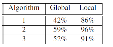
Now it is expected that the global R2 will be lower than it is on a local level. This shows another challenge in this: finding universal locations. Since EEM measures fluorescence, it is also influenced by the seasonality and geographical location of the sample, among other factors. For this reason, EEM may be viable, but there most likely won’t be universal predictors that extend across geography and seasons. In order to compensate for this, in practice, each water treatment facility would have to train their own model to account for the abnormalities from their geography
and seasonality.
We also sought to compare our methods to established techniques of variable selection and dimension reduction. However, many of those didn’t work with our data because of our small sample size, and it would have been beyond the scope of this project to explore other techniques. For example, when comparing our methods with Random Forests, we had difficulty using Random Forests techniques in a meaningful way because of the dependencies of our covariates.
Conclusion
EEM can be used to predict BOD, but there are clear drawbacks. Specifically, EEM varies due to the composition of its source waters, geography, and seasonality. For this reason, it makes robust inference more difficult. For a specific location, though, it could be used. Thus in practice, where we’re trying to use EEM to predict BOD to enable real-time monitoring of water pollution events, the model would need to be trained for the specific conditions. Also, another possible use of this was for developing countries where BOD technologies aren’t plausible due to cost. In a situation like this, it would be difficult because we may need to have BOD measures for that area, unless we find some proxy
measures for BOD since EEM depends on geography and seasonality.
Scholarly Sources
Coble, P., 1996. Characterization of marine and terrestrial DOM in seawater using excitation-emission matrix spectroscopy. March, pp. 325-46.
Galinha, C. F. et al., 2011. Two-Dimensional Fluorescence as a fingerprinting tool for monitoring wastewater treatment systems. Society of Chemical Industry, 14 Feb, pp. 985-991.
Hudson, N., Baker, A. & Reynolds, D., 2007. fluorescence analysis of dissolved organic matter in natural, waste and polluted waters. Wiley InterScience, 3 April, pp. 631-649.
Hudson, N. et al., 2007. Can fluorescence spectrometry be used as a surrogate for the Biochemical Oxygen Demand (BOD) test in water qualityassessment? An example from SouthWest England. Science for the Total Environment, 4 Dec, pp. 150-157. kaka, p., fififi, n., bobb, k. & nando, p., 2014. the act of love. big head, pp. 20-21.