
Alexander Poulsen and Brigham Frandsen, Economics
Introduction
Quantile instrumental variables estimators are a relatively new development in the econometric literature. Modern quantile regression was introduced in Koenker and Basset (1978), and has been used in many important applications in which researchers are interested in learning about the effects of variables on the distribution of an outcome variable, rather than just mean effects. Examples of these applications include changes in U.S. wage structure (Buchinsky 1994), the effect of school quality on student performance (Eide and Showalter 1998), and the relationship between innovation and firm growth (Coad and Rao 2008).
In these and other applications, regular OLS can give misleading results. For example, it could be that a certain policy has a large effect on lower income groups, but little or no effect on middle and upper income groups. In this case, a researcher using OLS would erroneously conclude that there was some small effect on all points of the distribution ⎯or perhaps no statistically significant effect at all⎯ rather than there being large effects on low income groups and little effect elsewhere. Results of this kind can have important policy implications, especially as social scientists are increasingly striving to understand and remedy inequality in education, income, and overall quality of life throughout the world.
Many of the important empirical questions we seek to answer in economics become difficult due to endogeneity of regressors. In layman’s terms, often x affects y and y in turn affects x, thus there is a feedback effect and it is difficult to identify the true effect of x on y. Econometricians began to make progress in adapting quantile regression models to deal with these problems in the early 2000s. Abadie, Angrist, and Imbens (2002) developed an estimator for quantile treatment effects with endogeneity and applied it to look at the effect of JTPA training on the distribution of earnings. Chernozhukov and Hansen (2004) developed a model quantile instrumental variable regression and applied it to look at how 401(k) participation affects wealth distribution. In this paper, I will compare these two methods to the Inverted CDF Estimator (henceforth, ICE) method outlined by Frolich, Melly (2008) and Frandsen (2015).
Methodology
I will compare these 3 estimators through monte carlo simulation. In monte carlo simulation, I create an artificial data-‐generating process for which I know what the true estimates are. I then run this simulation 2,000 times for each sample size, instrument strength and quantile combination for the 3 estimators. Through this repeated simulation, I am able to compare the estimators to each other by looking at statistics such as the bias, mean squared error, variance, and standard error coverage.
Results
I did the monte carlo analysis for 5 different quantiles (tau) and for 3 different sample sizes (n), so there are a lot of results. In this report I will only include one table that is illustrative of how the results look and are interpreted. The letter gamma in the table below signifies the strength of the instrumental variable. Lower values for gamma mean a weaker instrument.
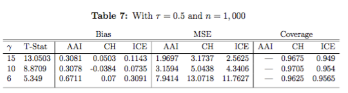
Across different sample sizes, I found that the standard errors for the Chernozhukov and Hansen estimator were on average not big enough for extremal quantiles. I also found that the mean squared error (MSE) of the CH was not only higher than the other estimators, but that it gets increasingly bigger when the instrumental variable is weak. The ICE I found to be generally less biased that the other two estimators.
Discussion
The finding that CH standard errors were too small for extremal quantiles means that using this estimator, you my find statistically significant results that are not actually statistically significant. The MSE gives an idea of how spread out the simulations are from each other, and is a good measure of how biased estimates are on average, so CH is on average more biased than the other estimators.
Conclusion
The most important results I have found are with respect to the Chernozhukov and Hansen estimator. One important thing to highlight is the fundamental difference between CH and the other two estimators. CH is an estimator that can compute quantile regressions of an outcome on any regressor, whereas the other two estimators can only calculate treatment effects, or in other words, only work with binary regressors. So given these findings, if you do not have a binary regressor, CH is your only option; however, if you have a binary regressor, you would be better off using ICE or AAI.