
Evan Magnusson and Richard Evans, Economics Department
Introduction
The goal of this project was to analyze the consequences of income tax cuts on government revenues. We did so using a large overlapping generations (OLG) model. This model was calibrated to closely match the distribution of labor, income, and wealth in the U.S. economy across both heterogeneous age and ability groups. By using a dynamic model, we were able to take into account the macroeconomic feedback effects that are absent from some analyses of tax proposals. We found that while our income tax cut was not completely self-financing, about forty three percent of a ten percent decrease in the income tax pays for itself.
Methodology
In order to use dynamic scoring to analyze these tax cuts, we built an overlapping generations model. This allowed changes in fiscal policy to affect wage and interest rates, labor participation rates, and GDP. Changes in these macroeconomic variables would in turn influence government revenues. These macroeconomic feedback effects were vital to an accurate analysis of the effect of a ten percent decrease in the income tax on government revenues.
Our model has a complex household side of the model and very simple firm and government sides. Individual households derive utility from consumption, leisure, and giving bequests throughout their entire life (i.e., both incidental and accidental bequests are permitted). In order for our model to be able to analyze distributional effects of tax changes, households differ by age and ability. We use eighty different age groups (representing ages 21 through 100) and seven different ability groups (representing the top 25th, 50th, 70th, 80th, 90th, 99th, and 100th income percentile groups). The first step in building the model was to program a very simple version of the household and firm sides of the economy, with no taxes or government. We then made the household side increasingly complex, testing the code as we went to make sure that everything functioned properly. One of these additions was to use an ellipse to fit the CRRA utility function for labor to assist in decreasing the computational complexity of the model. Demographics were added to the model using US data for fertility, mortality, and immigration rates from 2010 CDC, SSA, and Census data, respectively. Due to a nonzero growth rate in the model after implementing these realistic demographics, the model was stationarized. Finally, a government side was added to the model, where the government only taxes households (and returns tax revenues equally to households as a lump sum transfer). Only payroll and income taxes were used in this analysis, however.
In order to have our model accurately reflect the effects of the tax changes in the US economy, the model was calibrated to match the income, wealth, and labor distribution in the US. To do this, we used data from the Consumer Population Survey and US Treasury. The income tax was also calibrated to match the US’s current marginal tax rates using the IRS SOI program. The calibration process was very computationally intense, in particular because matching the top percentile group’s wealth holdings is very difficult. Once we calibrated the model to match the wealth, labor, and income distributions, we ran the model twice, once with the current income tax code structure to get a baseline steady state and transition paths values for our variables of interest, and then again with the tax change. We then used the output from these two simulations to judge the overall effects of the change.
Results and Discussion
As expected, decreasing the income tax burden by ten percent increases the steady state capital stock, labor, consumption, and output. The aggregate capital stock increased by 1.1%, aggregate effective labor rose by 0.29%, aggregate consumption rose by 0.43%, and aggregate output increased by 0.26%. Government revenues, as expected, decreased. However, they only fell by 6.7 percent. Thus, about 43% of the income tax cut is self-financing. In their simplified model, Mankiw and Weinzierl (2006) showed that about half of a capital income tax cut pays for itself. Figure 1 illustrates the transition path from the steady state before the tax change to the steady state after the change.
Conclusion
Our result is significant for a few reasons. One, it verifies Mankiw and Weinzierl’s (2006) result that tax cuts can help pay for themselves, at least in part. However, the difference between our results and Mankiw and Weinzierl’s are likely due to the more complex model we have implemented, as well as its highly detailed calibration. Finally, our results show that dynamic scoring should be used when evaluating the effects of tax policies, as ignoring the macroeconomic feedback effects involved with changes in fiscal policy make the policies seem more costly than they might be when implemented.
References
- Mankiw, N. Gregory, and Matthew Weinzierl. “Dynamic Scoring: A Back-of-the-envelope Guide.” Journal of Public Economics 90, no. 8-9 (2006): 1415-433.
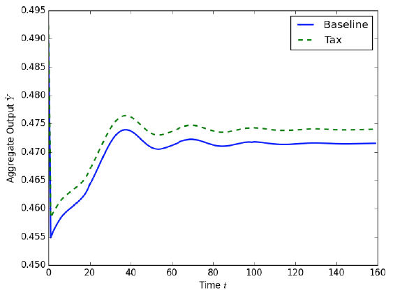
Figure 1 – This is the time path of aggregate output when going from the steady state with the original income tax levels to the steady state with the income tax cuts. As is seen, after implementing the policy change, output increases in every future period. Studying these time paths is useful, because if output increased 100 years from now, but plummeted until then, it might not be an advisable policy change.